
Embark on a mathematical journey with logistic growth ap calculus bc, where we delve into the intricacies of population growth and decay, unraveling the secrets of carrying capacity and maximum growth rates. Join us as we explore the applications of this fascinating concept in fields ranging from ecology to economics.
From deriving differential equations to analyzing inflection points, we’ll provide a comprehensive understanding of logistic growth, empowering you to tackle complex problems with confidence.
Logistic Growth Function
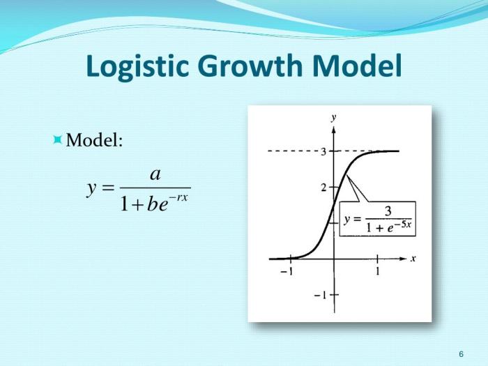
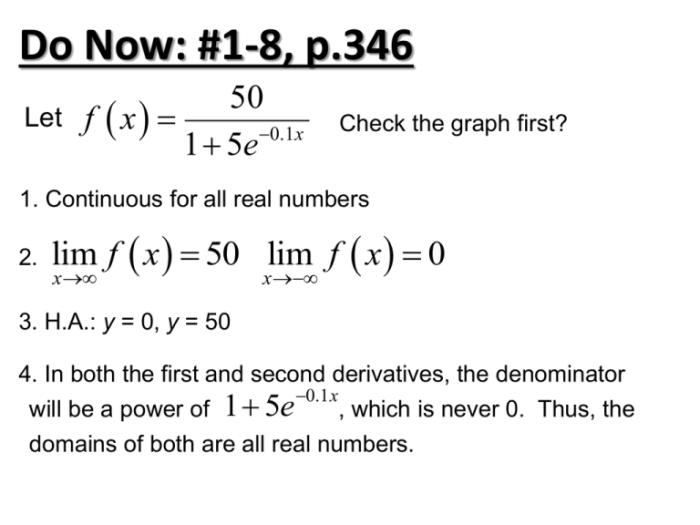
The logistic growth function is a mathematical model that describes the growth of a population over time. It is a sigmoid curve that starts slowly, then accelerates, and finally levels off as the population approaches its carrying capacity.
Equation of the Logistic Growth Function
The equation of the logistic growth function is:
P(t) = $\fracL1 + e^-kt$
where:
- P(t) is the population size at time t
- L is the carrying capacity
- k is the growth rate
Examples of Logistic Growth Function
The logistic growth function can be used to model a variety of real-world scenarios, including:
- The growth of a population of bacteria
- The spread of a disease
- The growth of a company’s market share
Significance of the Carrying Capacity
The carrying capacity is the maximum population size that can be supported by a given environment. It is a critical parameter in the logistic growth function because it determines the upper limit of the population’s growth.
Differential Equation of Logistic Growth
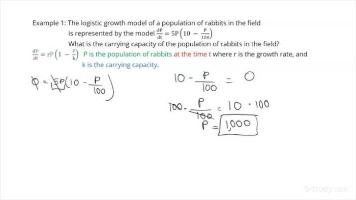
The differential equation that describes logistic growth is derived from the assumption that the rate of population growth is proportional to the population size and the amount of resources available.
Mathematically, this can be expressed as:
$$\fracdPdt = kP(1
\fracPK)$$
where:
- $P$ is the population size at time $t$
- $k$ is the growth rate
- $K$ is the carrying capacity
The relationship between the differential equation and the logistic growth function is that the logistic growth function is a solution to the differential equation.
The differential equation can be used to analyze logistic growth by finding the equilibrium points and determining their stability.
Equilibrium Points, Logistic growth ap calculus bc
The equilibrium points of the differential equation are the values of $P$ for which $\fracdPdt = 0$.
There are two equilibrium points:
- $P = 0$
- $P = K$
Stability of Equilibrium Points
The stability of an equilibrium point is determined by the sign of $\fracd^2Pdt^2$ at that point.
- If $\fracd^2Pdt^2< 0$, then the equilibrium point is stable.
- If $\fracd^2Pdt^2 > 0$, then the equilibrium point is unstable.
For the logistic growth differential equation, we have:
$$\fracd^2Pdt^2 = kP(1
\frac2PK)$$
At $P = 0$, $\fracd^2Pdt^2 = kP > 0$, so $P = 0$ is an unstable equilibrium point.
Logistic growth in AP Calculus BC is a fascinating concept that models population growth with a carrying capacity. Like the Santa Maria Ilocos Sur Church , which is a historical landmark in the Philippines, logistic growth curves reach a steady state, highlighting the importance of understanding population dynamics in calculus.
At $P = K$, $\fracd^2Pdt^2 = -kP< 0$, so $P = K$ is a stable equilibrium point.
Inflection Point and Maximum Growth Rate: Logistic Growth Ap Calculus Bc

The inflection point and maximum growth rate are crucial characteristics of the logistic growth function, providing valuable insights into the dynamics of population growth.
Inflection Point
The inflection point is the point on the logistic growth curve where the function changes from concave up to concave down. Mathematically, it occurs when the second derivative of the function is zero. The inflection point represents the transition from a period of rapid growth to a period of slower growth.
Maximum Growth Rate
The maximum growth rate is the maximum value of the first derivative of the logistic growth function. It represents the steepest slope of the curve and corresponds to the point of maximum population growth.
The inflection point and maximum growth rate are closely related. The maximum growth rate occurs at half the carrying capacity, which is the inflection point.
Applications of Logistic Growth
Logistic growth is a fundamental concept used in various fields to model and predict the growth of populations and systems that follow a sigmoid curve. It finds applications in fields such as population ecology, epidemiology, economics, and resource management.
Population Ecology
In population ecology, logistic growth is used to model the growth of populations of organisms. The carrying capacity of the environment, which represents the maximum population size that can be sustained, plays a crucial role in shaping the population’s growth trajectory.
Logistic growth helps ecologists predict population dynamics and understand the factors that influence population growth rates.
Epidemiology
In epidemiology, logistic growth is used to model the spread of infectious diseases. The model considers factors such as the rate of infection, the recovery rate, and the population’s immunity levels. By understanding the logistic growth pattern, epidemiologists can make predictions about the course of an epidemic and implement effective control measures.
Economics
In economics, logistic growth is used to model the growth of industries, markets, and technological adoption. It helps economists understand the dynamics of market penetration and forecast future trends. By analyzing the logistic growth curve, economists can make informed decisions about investment strategies and resource allocation.
Limitations and Challenges
While logistic growth is a powerful tool for modeling growth phenomena, it has limitations and challenges:
-
-*Assumptions
Logistic growth assumes that the growth rate is proportional to both the population size and the carrying capacity. This assumption may not always hold true in real-world scenarios.
-*Environmental Fluctuations
Real-world populations and systems are subject to environmental fluctuations and stochastic events that can deviate from the smooth logistic growth curve.
-*Parameter Estimation
Accurately estimating the parameters of the logistic growth function, such as the carrying capacity and growth rate, can be challenging, especially in complex systems.
FAQ Guide
What is the logistic growth function?
The logistic growth function is a mathematical equation that describes the growth of a population over time, taking into account both growth rate and carrying capacity.
How is the logistic growth function used in real-world scenarios?
The logistic growth function is used in a wide range of fields, including population ecology, epidemiology, and economics, to model the growth and decline of populations.
What is the significance of the carrying capacity in the logistic growth function?
The carrying capacity represents the maximum population size that can be supported by the available resources in a given environment.

